Hedonic Home Price Prediction
In Boston, the house market is thriving. Housing price prediction is important to prospective homeowners, developers, investors and other real estate market participants.
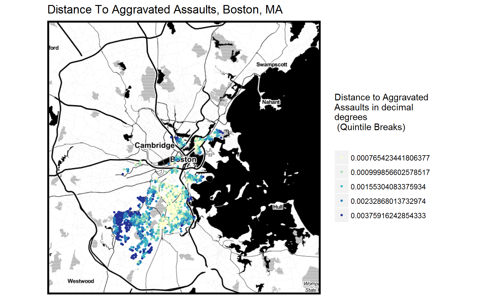
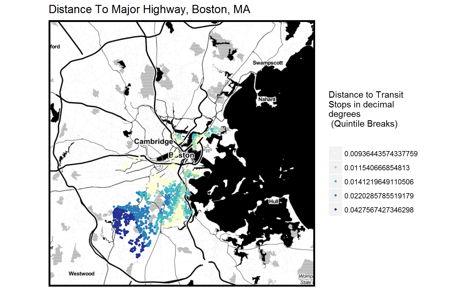
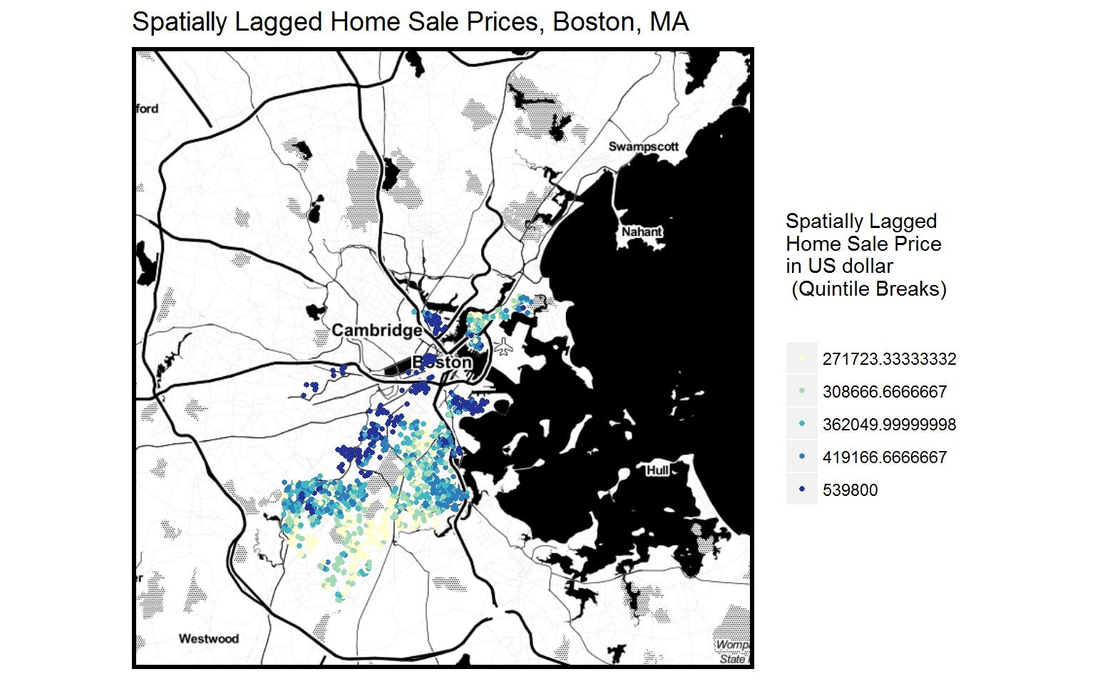
3 most Interesting Predictor Variables
- Distance to aggravated assaults
- Distance to transit stops
- Sptially lagged home prices
- Distance to aggravated assaults
- Distance to transit stops
- Sptially lagged home prices
Zillow Group, an online real estate database company, has realized that its housing market predictions are not as accurate as they could be due to insufficient local intelligence, so they have required us to build a better OLS regression model to predict home sale prices for Boston.
In our model, the dependent variable is home sale prices, and we consider three main categories of decision factor: internal characteristics, amenities and public services, and the underlying spatial structure of prices. See below for all selected predictors.
Note: in all the regressions we conduct, we actually use the logarithmic transformation of the home sale price instead of the raw values of the sale prices, since the dependent variable home sale prices are not normally distributed.
List of Predictors
- “SalePrice”: the home sale price point in Boston of our dataset. (Note: in the OLS regression model we conduct for our analysis, we take a logarithmic transformation of the values of the home sale price, since the raw values of the home sale price are not normally distributed)
- “d_transit”: the average distance between each home sale price point of our dataset and its 5 nearest MBTA transit stops.
- “d_crime”: the average distance between each home sale price point of our dataset and its 5 nearest aggravated assault points.
- “d_schools”: the average distance between each home sale price point of our dataset and its 5 nearest colleges or universities.
- “d_hwy”: the distance for each home sale price point to its nearest major highway in Boston.
- “WT_SP”: the spatial lag of each home sale price. That is, the average sale price of each home sale price point’s 5 nearest sale prices. (Note: in the OLS regression model we conduct for our analysis, we take a logarithmic transformation of the spatial lag variable of home sale prices, since the raw values of the spatial lag variable are not normally distributed)
- “NAME10”: the census tract in which each home sale price locates.
- “Style”: the house style of each home sale price point (i.e. decker, row end, and conventional).
- “LU”: Land use and zoning type for each home sale price point(i.e.R1: single family residence ).
- “GROSS_AREA”: the gross living area of each home sale price point.
- “NUM_FLOORS”: the number of floors for each home sale price point.
- “R_ROOF_TYP”: the roof type of each home sale price point (i.e. F: flat roof, M: Mansard roof).
- “R_EXT_FIN”: the exterior finishing material of each home sale price point(i.e. B: brick, W: wood).
- “R_TOTAL_RM”: the total number of rooms for each home sale price point.
- “R_BDRMS”: the number of bedrooms for each home sale price point.
- “R_FULL_BTH”: the number of full size bathrooms for each home sale price point.
- “R_HALF_BTH”: the number of half size bathrooms for each home sale price point.
- “R_KITCH”: the number of kitchens for each home sale price point.
- “R_HEAT_TYP”: the types of heating systems for each home sale price point(i.e. E: Electric Space Heaters, W: Wood-Burning and Pellet Stoves).
- “R_AC”: the types of air conditioning systems for each home sale price point.
- “YR_BUILT_RC”: the year of each home sale price point was built.
- “YR_REMOD_RC”: the year of each home sale price point was remodeled.
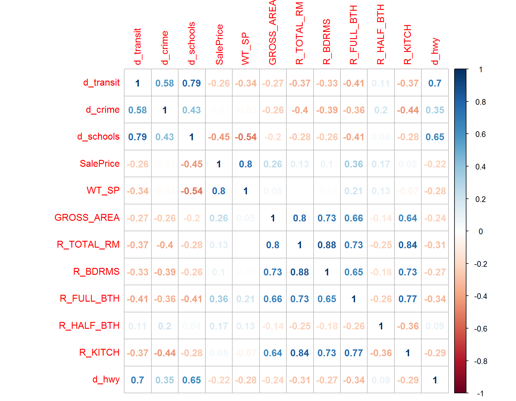
Correlation Matrix
We analyze the pairwise correlations between these predictor variables. This helps us evaluate how inter-correlated these predictors are. The higher the absolute correlation value, the more inter-correlated between the two predictors.
In-Sample Regression
Our in-sample regression result shows that our model explains approximately 90% of the variance in the dependent variable home sale prices (R-Squared: 89.5). The Mean Absolute Percentage Error (MAPE), a measure of prediction accuracy of a forecasting method, has a value of around 11% for the in-sample prediction.
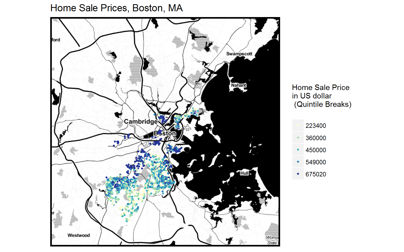
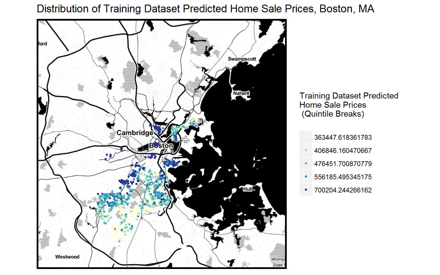
Distribution of Home Prices
- Original
- Predicted (training)
- Predicted (test)
- Original
- Predicted (training)
- Predicted (test)
Out-of-Sample Regression
Since we obviously do not know the future home sale prices in Boston, we need to simulate the out-of-sample usefulness of the model by separating the home sale price data into a training set that we use to train the model and a test set that we use to validate our model. Thus, we randomly select 75% of the home sale price observations from the data as our training set and the other 25% sale price observations is our test set to see how generalizable the model is.
We first build an OLS regression model of the training set with the same predictors as our in-sample regression model. Then we use the training set regression model to predict the home sale prices of the test set.
The two maps above compares the distribution of original home prices and the predicted training dataset home prices. Visually they display similar spatial patterns.
Summary of Out-of-Sample Regression Result
- R-squared
- Root mean square error(RMSE)
- Mean absolute error(MAE)
- Mean absolute percent error(MAPE)
- R-squared
- Root mean square error(RMSE)
- Mean absolute error(MAE)
- Mean absolute percent error(MAPE)
Moreover, we use the RMSE, MAE and MAPE of the randomly selected test set to see how much our predicted values are different from the observed home sale prices and understand how well our model predict.
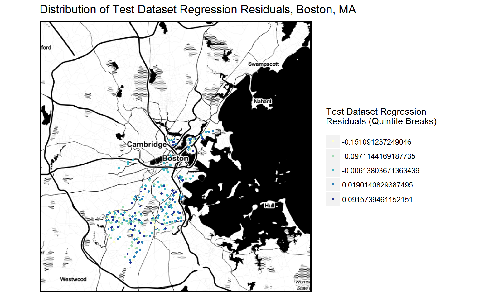

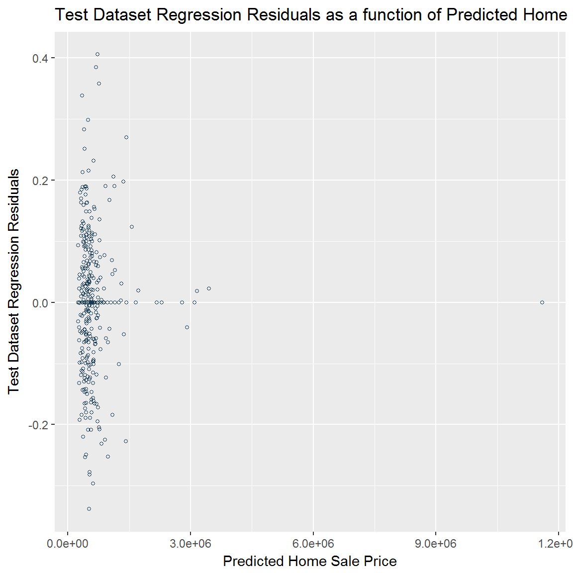
Test Dataset Regression Residuals (Errors)
- Spatial distribution
- As a function of observed home price
- As a function of predicted home price
- Spatial distribution
- As a function of observed home price
- As a function of predicted home price
The map on the left above showing the distribution of test dataset regression residuals allows us to further examine if our model sucessfully addresses spatial factors. The test dataset regression residuals are constantly distributed acrross space, revealing that there is little spatial autocorrelation in test dataset regression residuals.
The Moran’s I test results confirm our interpretation of the map. The close-to-1 and slightly negative Moran’s I value (-0.11) indicates little spatial autocorrelation.
We also plot the test dataset regression residuals as a function of the observed and predicted values of home sale price. These plots allow us to examine visually the generalization of the model.
We also plot the test dataset regression residuals as a function of the observed and predicted values of home sale price. These plots allow us to examine visually the generalization of the model.
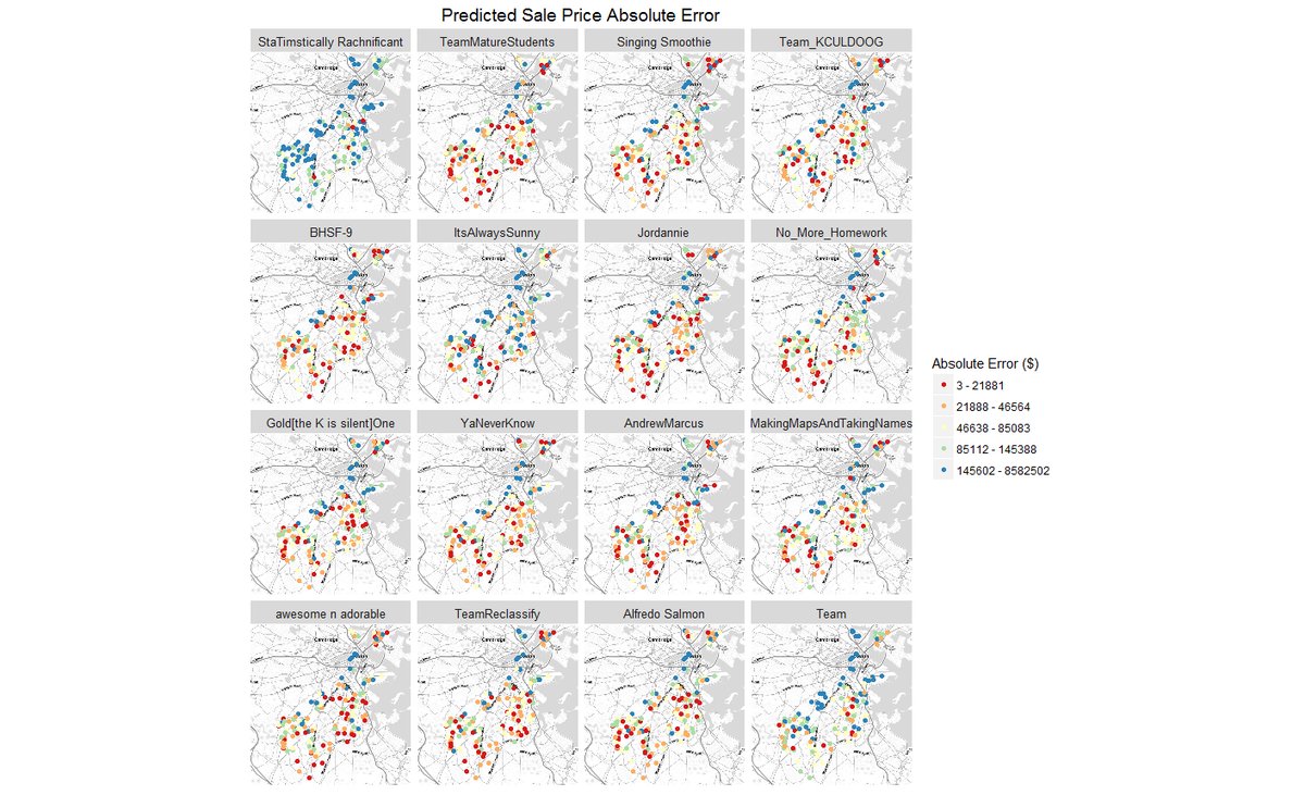
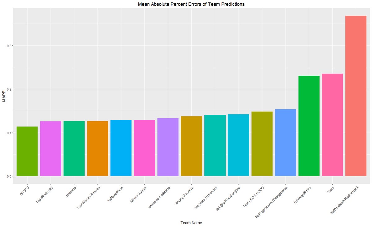
Class Contest Result
- 1st price among 12 groups
- Cr to Ken Steif (MUSA 507 Instructor + MUSA Director)
- 1st price among 12 groups
- Cr to Ken Steif (MUSA 507 Instructor + MUSA Director)
This class project is also a class contest. We are “TeamReclassify”. On the MAPE plot, we rank 2nd place, but in fact after our instructor checked with the first team, they found a predictor not appropriate to use, so we are the one that won the contest in the end. Below is the contest description.
“Winning the contest is all about predictive accuracy. The winning team will be the one that is able to do two things. First, to find the best predictive ‘features’ or variables. Second, pour enough predictive power into the model to predict well without overfitting. You want to create a model that is ‘generalizable’ to the many different neighborhoods in Boston.”
Limitations
There are some limitations of our model. Our model may predict better for rich neighborhoods than for poor neighborhoods due to our selected predictors. Hence, we can add some more predictors which have more explanatory power in poor neighborhoods or in a comprehensive scale in Boston, such as median household income, employment rate and ethnicity factors.